Short answer
SQL order of execution is logical: FROM/JOIN, WHERE, GROUP BY, HAVING, SELECT, DISTINCT, ORDER BY, LIMIT. Physically, the engine parses, rewrites, plans with a cost model, then executes the chosen plan and returns rows.
On this page
- What is the logical order of a SQL query?
- Why can’t I use a SELECT alias in WHERE?
- What is the difference between WHERE and HAVING?
- Why do window functions need a subquery or QUALIFY?
- What mistakes does this order explain?
- What does the database actually do with a query?
- How do other engines differ?
- What should you take from the two layers?
The short version
- The SQL order of execution is a logical model: FROM and JOIN, WHERE, GROUP BY, HAVING, SELECT, DISTINCT, ORDER BY, then LIMIT. It decides which names each clause can see.
- Microsoft Learn lists 12 logical steps for SELECT and says the query processor decides the actual physical order, which can differ.
- PostgreSQL’s documented path has five stages: connection, parser, rewrite system, planner/optimizer, executor.
- The planner is cost-based. It builds candidate paths, such as a sequential scan or an index scan, estimates each, and keeps the cheapest.
- Window functions run after WHERE, GROUP BY and HAVING. To filter them, use a subquery, or QUALIFY in Snowflake, BigQuery, DuckDB and Databricks. PostgreSQL has no QUALIFY.
- EXPLAIN shows the plan. EXPLAIN ANALYZE runs the query and adds real row counts and times per node.
SQL order of execution has two layers, because a SQL query has two lives. On paper, it is evaluated clause by clause in a fixed logical order. Inside the database, it is parsed, rewritten, planned and executed by code that is free to do the work in a different order, as long as the answer matches. Most articles on SQL order of execution only cover the first life. This one covers both and keeps them apart, because mixing them up causes many confusing SQL errors.
This explainer is part of Numeracy’s SQL tools, priced and compared, an independent guide to the data stack. If you pick your tools around query plans, our SQL editors compared hub covers the clients that can show them.
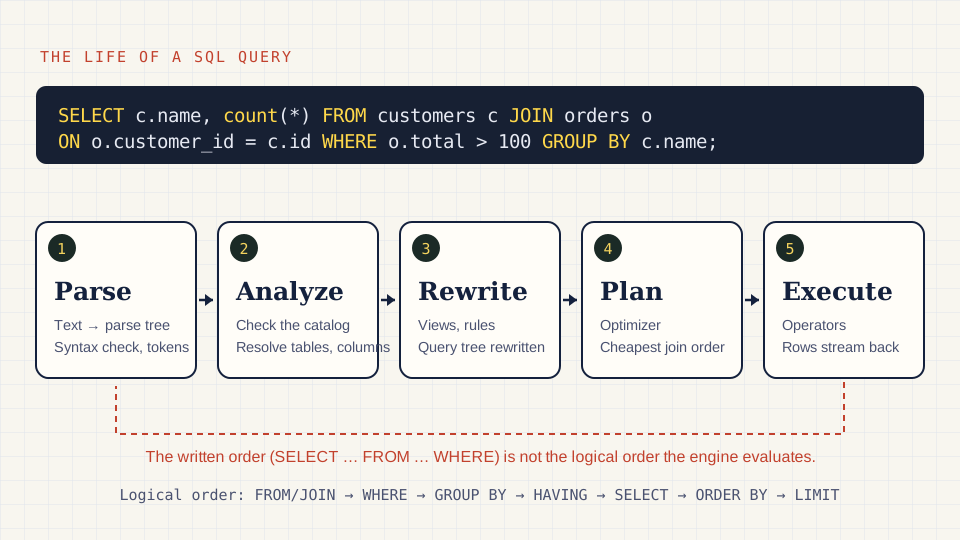
Swipe sideways to see the whole figure, or open it full size.
What is the logical order of a SQL query?
The logical order is the sequence in which clauses are conceptually evaluated, which fixes what each clause is allowed to reference. For a plain SELECT it runs FROM and JOIN, WHERE, GROUP BY, HAVING, window functions, SELECT, DISTINCT, ORDER BY, and finally LIMIT.
Microsoft Learn documents this for SQL Server as the “logical processing order, or binding order”. Its list has twelve steps: FROM, ON, JOIN, WHERE, GROUP BY, WITH CUBE or WITH ROLLUP, HAVING, QUALIFY (Fabric Data Warehouse only), SELECT, DISTINCT, ORDER BY and TOP. The page states the purpose plainly: the order determines when objects defined in one step become available to later steps. It then adds the caveat that matters for the second half of this article: the query processor determines the actual physical execution, and the order might vary.
BigQuery’s reference describes the same shape. Its syntax page says a query is completed in a stated order, with WINDOW before QUALIFY, and QUALIFY before DISTINCT, ORDER BY and LIMIT. It also notes that evaluation order does not always match syntax order, which is the whole reason SQL feels backwards: you write SELECT first, but it runs near the end.
A worked example on a toy dataset
This is a made-up example, small enough to follow by hand. It is not real data. There are two tables.
customers: id 1 is Ana (UK), id 2 is Ben (US), id 3 is Cy (US), id 4 is Di (UK).
orders: six rows, shown below as they enter the query.
| order id | customer id | amount | status |
|---|---|---|---|
| 101 | 1 | 40 | paid |
| 102 | 1 | 60 | paid |
| 103 | 2 | 25 | refunded |
| 104 | 2 | 80 | paid |
| 105 | 3 | 15 | paid |
| 106 | 4 | 90 | paid |
The question: which countries have more than 100 in paid revenue, biggest first?
SELECT c.country,
       COUNT(*)      AS paid_orders,
       SUM(o.amount) AS revenue
FROM orders o
JOIN customers c ON c.id = o.customer_id
WHERE o.status = 'paid'
GROUP BY c.country
HAVING SUM(o.amount) > 100
ORDER BY revenue DESC
LIMIT 5;
Here is the row set after each logical step.
| Step | Clause | Row set after the step |
|---|---|---|
| 1 | FROM + JOIN … ON | 6 rows: every order joined to its customer, so each carries a country (UK: 101, 102, 106; US: 103, 104, 105) |
| 2 | WHERE | 5 rows: order 103 is removed (refunded) |
| 3 | GROUP BY | 2 groups: UK holds orders 101, 102, 106; US holds 104, 105 |
| 4 | HAVING | 1 group: UK sums to 190 and stays; US sums to 95 and is dropped |
| 5 | SELECT | 1 row: UK, paid_orders 3, revenue 190. The aliases paid_orders and revenue are created here |
| 6 | DISTINCT | not used in this query; it would remove duplicate output rows here |
| 7 | ORDER BY | 1 row, sorted by revenue, which exists now |
| 8 | LIMIT | 1 row, since 1 is below the limit of 5 |
Toy data defined for this article. Clause order per Microsoft Learn and BigQuery docs, checked Nov 17, 2026.
The US group never reaches SELECT, since HAVING removed it first. And revenue only exists from step 5 onward.
Why can’t I use a SELECT alias in WHERE?
Because WHERE runs before SELECT, so the alias has not been created yet. Microsoft Learn spells it out: since SELECT is a later step, column aliases it defines can’t be referenced by preceding clauses, but later clauses such as ORDER BY can use them.
PostgreSQL’s SELECT reference agrees and adds detail. An output column’s name can be used in ORDER BY and GROUP BY, but not in the WHERE or HAVING clauses; there you must write out the expression instead. Two edge rules from the same page apply. If a name matches both an input column and an output column, ORDER BY takes the output column and GROUP BY takes the input column. And an ORDER BY applied to a UNION, INTERSECT or EXCEPT can only use output names or numbers, not expressions.
Alias rules vary by engine, so treat “ORDER BY can see aliases” as the portable part and anything beyond it as something to check in your database’s docs. DuckDB’s docs, for example, show QUALIFY referring to a window function by its SELECT alias, which is a looser rule than the one PostgreSQL applies to WHERE and HAVING.
What is the difference between WHERE and HAVING?
WHERE filters rows before grouping. HAVING filters groups after aggregation. That is why aggregates are allowed in HAVING and rejected in WHERE: at the WHERE step, no groups exist.
In the toy example, HAVING SUM(o.amount) > 100 could not be a WHERE condition. But o.status = 'paid' belongs in WHERE even though HAVING could technically hold it in some queries. Filtering early means the grouping step sees five rows instead of six. On a real table, that is the difference between aggregating the rows you need and aggregating everything, then discarding.
Why do window functions need a subquery or QUALIFY?
Window functions are computed after WHERE, GROUP BY and HAVING, so those clauses can’t reference them. (The SQL window functions cheat sheet covers the syntax and which engines support QUALIFY.) The PostgreSQL tutorial says this directly: window functions are forbidden in GROUP BY, HAVING and WHERE since they logically execute after those clauses. It also says a row removed by WHERE is never seen by any window function, and that window functions execute after non-window aggregates.
To filter on a window result, PostgreSQL’s own tutorial shows wrapping it in a sub-select:
SELECT customer_id, order_id, amount
FROM (
  SELECT customer_id, order_id, amount,
         ROW_NUMBER() OVER (PARTITION BY customer_id ORDER BY amount DESC) AS pos
  FROM orders
) AS ranked
WHERE pos = 1;
Several engines add a clause for exactly this. QUALIFY filters the output of window functions the way HAVING filters aggregates. Snowflake’s docs place it after HAVING and the WINDOW clause and before DISTINCT, ORDER BY and LIMIT. BigQuery requires a window function in either the QUALIFY clause or the SELECT list. DuckDB describes it as a way to avoid a subquery or WITH clause. Databricks requires at least one window function in SELECT or QUALIFY and bars aggregates inside QUALIFY. Microsoft’s SELECT page lists QUALIFY too, but only for Fabric Data Warehouse. PostgreSQL’s SELECT page has no QUALIFY clause, so use the subquery there.
-- Snowflake, BigQuery, DuckDB, Databricks
SELECT customer_id, order_id, amount
FROM orders
QUALIFY ROW_NUMBER() OVER (PARTITION BY customer_id ORDER BY amount DESC) = 1;
What mistakes does this order explain?
Most “why does this error out” questions come down to a clause asking for something that does not exist yet at its step. Here are five, each wrong then right. Interviewers test the same ideas, as our SQL interview questions for data analysts show.
1. Alias in WHERE
-- Wrong: revenue does not exist at the WHERE step
SELECT amount * 1.2 AS gross FROM orders WHERE gross > 100;

-- Right: repeat the expression
SELECT amount * 1.2 AS gross FROM orders WHERE amount * 1.2 > 100;
2. Aggregate in WHERE
-- Wrong: groups are not formed yet
SELECT customer_id FROM orders WHERE SUM(amount) > 100 GROUP BY customer_id;

-- Right: HAVING runs after GROUP BY
SELECT customer_id FROM orders GROUP BY customer_id HAVING SUM(amount) > 100;
3. Window function in WHERE
-- Wrong: window functions run after WHERE
SELECT * FROM orders WHERE ROW_NUMBER() OVER (ORDER BY amount DESC) <= 3;

-- Right: compute first, filter after
SELECT * FROM (
  SELECT *, ROW_NUMBER() OVER (ORDER BY amount DESC) AS rn FROM orders
) t WHERE rn <= 3;
4. Filtering the right side of a LEFT JOIN in WHERE
ON is evaluated with the join, and WHERE runs after it. A WHERE condition on the optional table throws away the NULL-extended rows the LEFT JOIN just kept, so the query behaves like an inner join.
-- Wrong: customers with no paid orders disappear
SELECT c.name, o.amount
FROM customers c
LEFT JOIN orders o ON o.customer_id = c.id
WHERE o.status = 'paid';

-- Right: keep the condition in ON to preserve customers without paid orders
SELECT c.name, o.amount
FROM customers c
LEFT JOIN orders o ON o.customer_id = c.id AND o.status = 'paid';
5. Selecting a column that is not grouped
-- Wrong: after GROUP BY country, each group has many customer ids
SELECT country, customer_id, COUNT(*) FROM customers GROUP BY country;

-- Right: select only grouped columns and aggregates
SELECT country, COUNT(*) FROM customers GROUP BY country;
PostgreSQL rejects the first form with an error. Some other engines accept it and return an arbitrary value, so check how yours behaves.
One more related to the end of the pipeline: LIMIT without ORDER BY. LIMIT is applied last, but if nothing orders the rows, which rows survive is up to the engine. PostgreSQL’s SELECT page says to use an ORDER BY that produces a unique order when you use LIMIT.
What does the database actually do with a query?
The database does not walk the clauses in order. It runs a pipeline. PostgreSQL’s documentation, which this section uses as its primary source, describes five stages in “The Path of a Query”.
- Connection. An application connects to the server, sends the query text and waits for results.
- Parser. The parser checks syntax and builds a query tree. The analysis of names and types is part of this front end, which is why a misspelled column fails before any data is read.
- Rewrite system. The rewriter takes the query tree and applies rules stored in the system catalogs. Its documented use is views: a query on a view, which is a virtual table, is rewritten into a query on the base tables in the view’s definition.
- Planner/optimizer. The planner takes the rewritten tree and creates a query plan for the executor.
- Executor. The executor recursively steps through the plan tree, retrieves rows, uses the storage system to scan relations, performs sorts and joins, evaluates qualifications and returns the rows.
The diagram above shows the same flow. The logical order from the first half is the meaning the parser and planner must preserve. The executor does not follow it as a schedule.
How does the planner choose a plan?
The planner generates candidate paths that give the same result, estimates a cost for each, and keeps the cheapest. The PostgreSQL docs give a plain example: a table with an index yields two scan paths, a sequential scan and an index scan.
The Planner/Optimizer page lists the building blocks:
- Scans. A sequential scan is always generated for each base relation. An index scan is generated when a restriction on a column matches an index and operator class. Index scans are also considered when an index’s sort order can satisfy an ORDER BY or help a merge join.
- Joins. Nested loop, merge join and hash join. A nested loop scans the right side once per left row and suits an indexed right side. A merge join sorts both sides on the join keys and scans each once. A hash join loads the right side into a hash table and probes it with the left.
- Join order. With fewer relations than
geqo_threshold, the planner searches nearly exhaustively. Above it, PostgreSQL switches to the Genetic Query Optimizer, which keeps planning time bounded and may not find the optimal order. - Filters and projections. The planner attaches WHERE conditions and output expressions to the most suitable plan nodes. This is why “WHERE runs before JOIN” is a model, not a rule of the machine: the planner can apply a filter at a scan below the join.
Estimates need data about data. Row estimates come from statistics that ANALYZE collects from a random sample of each table, so stale statistics can lead to a poor plan. SQLite’s query planner doc makes the same point about its own engine: once ANALYZE has gathered statistics, SQLite can prefer the index expected to narrow results most, and without them a choice between equally good indexes is arbitrary.
How does the executor run the plan?
The executor works on a tree of plan nodes. PostgreSQL’s description is that it steps recursively through the tree, so the top node asks its children for rows, and those ask theirs, down to the scans that touch storage. This pull-based, node-per-operator style is commonly called the iterator or Volcano model; the PostgreSQL page describes the recursive stepping rather than using that name, so treat the label as background, not a quote.
One consequence you can see in the plan below: a parent may stop reading early. The docs note that a node’s total cost assumes it runs to completion, but a parent such as LIMIT can stop sooner.
How do I read an EXPLAIN plan?
Run EXPLAIN in front of the statement. The next block is an illustrative plan for the toy query above, written to show the shape. The cost and row numbers are placeholders, not a measured result from any database.
Limit  (cost=A..B rows=1 width=..)
  ->  Sort  (cost=.. rows=.. width=..)
        Sort Key: (sum(o.amount)) DESC
        ->  HashAggregate  (cost=.. rows=.. width=..)
              Group Key: c.country
              Filter: (sum(o.amount) > 100)
              ->  Hash Join  (cost=.. rows=.. width=..)
                    Hash Cond: (o.customer_id = c.id)
                    ->  Seq Scan on orders o  (cost=.. rows=.. width=..)
                          Filter: ((status)::text = 'paid'::text)
                    ->  Hash  (cost=.. rows=.. width=..)
                          ->  Seq Scan on customers c  (cost=.. rows=.. width=..)
Read it from the most indented node outward, since that is where rows originate. According to the PostgreSQL docs, each node is one line, children are indented under their parent with ->, and the top line is the root. Here the two sequential scans feed a hash join. The WHERE condition appears as a filter on the orders scan, which is the planner applying it early. The HAVING condition appears as a filter on the aggregate node, since the aggregate must exist first. The sort and limit sit on top, matching the end of the logical order.
Each node carries (cost=startup..total rows=N width=W). Startup is the estimated cost before the first row can come out, total is the cost to finish, rows is the estimated output rows (not rows scanned), and width is the average row width in bytes. Costs are in arbitrary units, conventionally anchored to seq_page_cost = 1.0, so they compare plans against each other and are not milliseconds.
EXPLAIN ANALYZE executes the query and adds measured values. The PostgreSQL docs show this for a filtered scan:
EXPLAIN ANALYZE SELECT * FROM tenk1 WHERE ten < 7;

 Seq Scan on tenk1  (cost=0.00..470.00 rows=7000 width=244) (actual time=0.030..1.995 rows=7000.00 loops=1)
   Filter: (ten < 7)
   Rows Removed by Filter: 3000
Excerpt from the PostgreSQL documentation, Using EXPLAIN, checked Nov 17, 2026. Output trimmed.
Some clients draw the plan for you: pgAdmin has a graphical EXPLAIN tab, while DBeaver shows a table view, as our DBeaver vs pgAdmin comparison covers. Compare estimated rows with actual rows first. A large gap points to stale or missing statistics. Then check loops: for nodes that run more than once, the docs say the time and rows shown are per-execution averages, so multiply by loops. Last, remember that EXPLAIN ANALYZE really runs the statement. For an UPDATE or DELETE, the docs suggest wrapping it in a transaction and rolling back.
A SQL editor that shows the query plan visually makes this much faster to scan than raw text, especially for plans with many nodes. Our best SQL editor page compares clients on exactly those details, and the SQL clients dataset lists them with sourced prices.
How do other engines differ?
The logical model carries over; the physical machinery does not. Three documented examples:
- SQL Server. Microsoft publishes the logical processing order as a binding order and says the real execution can vary. Its SELECT page also gives a rare case where the sequence differs: a CONVERT in a view’s select list can execute before WHERE when the view has a clustered index.
- SQLite. Its planner doc describes the planner choosing between full table scans, rowid lookups and index lookups, and says indexes should change only how fast a result arrives, never the result.
- Columnar and distributed warehouses. BigQuery’s documentation says it converts SQL into an execution graph of stages that run in parallel on a distributed architecture, with slots doing the work. Snowflake’s Query Profile shows the execution plan as an operator tree where each node is a rowset operator with its share of total query time. The vocabulary is different, but you read these graphs the same way: find the expensive operator, then ask why the rows reaching it were so many.
I have not covered engine internals beyond what those pages state. If you need details such as exactly which join algorithms a given warehouse supports, check that vendor’s current docs.
What should you take from the two layers?
Use the logical order to write correct SQL and to decode errors. Use the physical path to understand why two logically identical queries can run at very different speeds. They answer different questions: the first says what a query means, the second says how a particular engine will produce that meaning today.
Questions people ask
What is the order of execution of a SQL query?
The logical order is FROM and JOIN, WHERE, GROUP BY, HAVING, window functions, SELECT, DISTINCT, ORDER BY, then LIMIT or TOP. Microsoft Learn lists twelve logical steps for SELECT and warns the engine decides the real physical order.
Why can I not use a column alias in the WHERE clause?
WHERE is evaluated before SELECT, so the alias does not exist yet. PostgreSQL documents that an output column name works in ORDER BY and GROUP BY but not in WHERE or HAVING. Repeat the expression, or wrap the query in a subquery.
What is the difference between WHERE and HAVING?
WHERE filters individual rows before grouping, so it cannot contain aggregates. HAVING filters whole groups after GROUP BY, so it can. Put row-level conditions in WHERE, which shrinks the input to the aggregation, and keep HAVING for conditions on aggregates.
How do I filter on a window function?
Window functions run after WHERE, GROUP BY and HAVING, so they are not allowed in those clauses. Compute the window function in a subquery or CTE and filter in the outer query. Snowflake, BigQuery, DuckDB and Databricks also offer QUALIFY; PostgreSQL does not.
Does the database really run clauses in that order?
No. The order is a model for deciding what each clause can see. The optimizer is free to reorder joins and push filters down as long as the result is the same. PostgreSQL docs describe a cost-based planner that picks the cheapest path.
What does EXPLAIN do in PostgreSQL?
EXPLAIN prints the plan the planner chose, with estimated cost, rows and width for each node. EXPLAIN ANALYZE runs the statement as well and adds actual time, rows and loops, so wrap data-changing statements in a transaction you roll back.
Sources
- PostgreSQL docs: The Path of a Query ·
- PostgreSQL docs: Planner/Optimizer ·
- PostgreSQL docs: Using EXPLAIN ·
- PostgreSQL docs: SELECT ·
- PostgreSQL docs: Window Functions tutorial ·
- Microsoft Learn: SELECT (Transact-SQL), logical processing order ·
- Snowflake docs: QUALIFY ·
- BigQuery docs: Query syntax, QUALIFY clause ·
- DuckDB docs: QUALIFY clause ·
- Databricks docs: QUALIFY clause ·
- SQLite docs: The SQLite Query Planner ·
- BigQuery docs: Query plan and timeline ·
- Snowflake docs: Query Profile ·